
Table of Contents
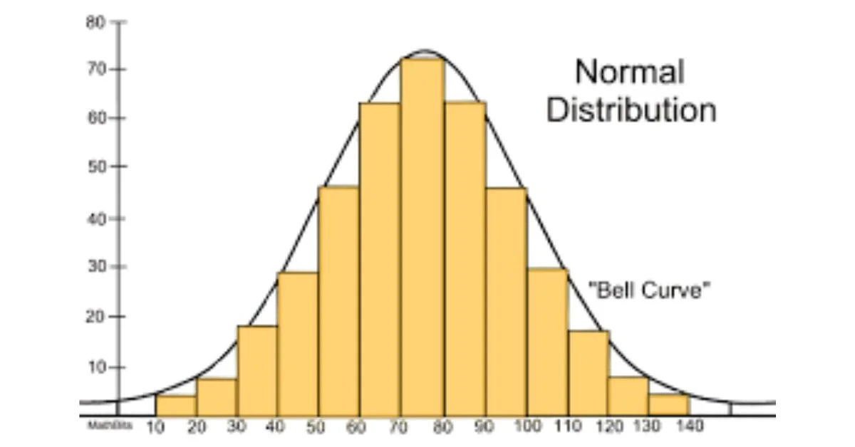
A normal distribution (also called a Gaussian distribution) is a way to describe how data clusters around an average. If you take a large set of measurements, like heights or test scores, and plot how often each value occurs, you often get a smooth, bell-shaped curve. Most values gather around the center, and fewer appear as you move away, creating a mirror image on both sides.
Why It Matters?
The normal distribution is everywhere:
- Heights of people.
- Test scores in a big class.
- Measurement errors in tools.
- Natural traits and many other things.
Because it’s so common, understanding normal distributions helps us make sense of data, predict outcomes, and find hidden patterns.
Key Properties
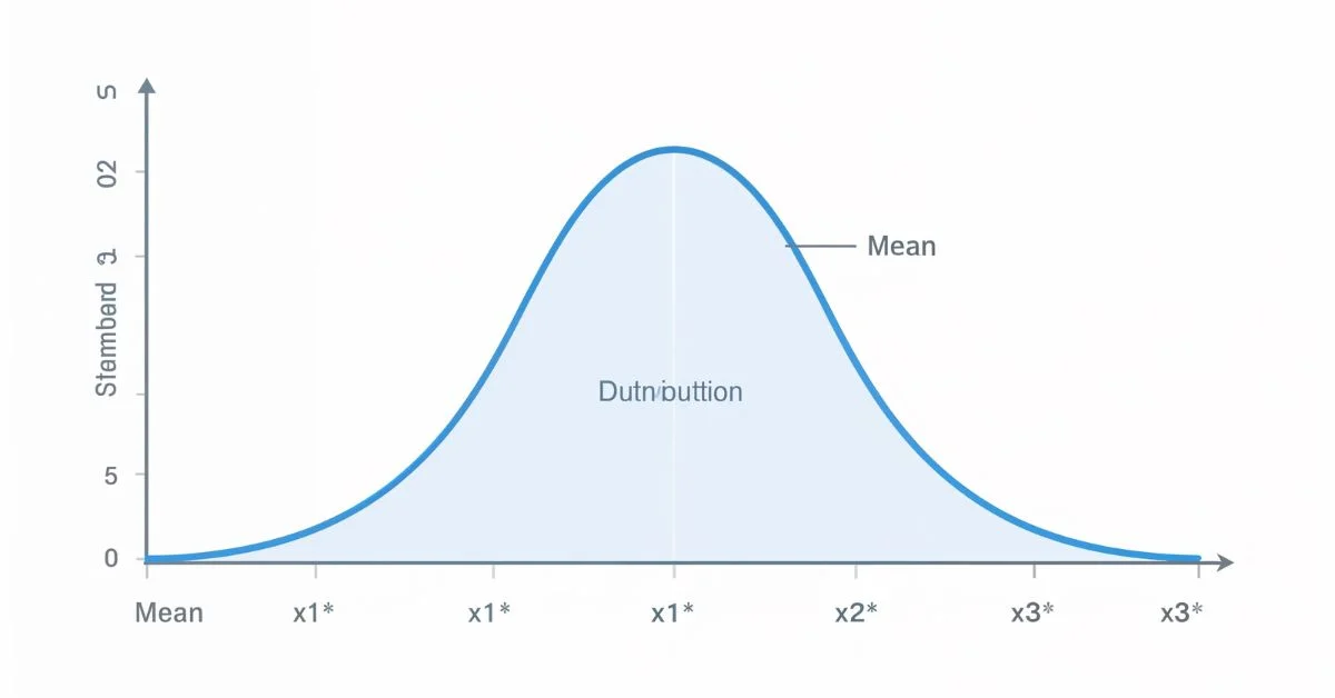
- Bell–shaped and symmetric: The curve is highest at the center and looks the same left and right.
- Mean = Median = Mode: The average, middle value, and most frequent value are all the same point.
- Defined by two numbers only: the mean (μ) tells where the center is, and the standard deviation (σ) shows how spread out the data are.
- Empirical Rule (68–95–99.7 rule):
-
- ~68% of the data lie within ±1σ from the mean.
- ~95% within ±2σ.
- ~99.7% within ±3σ.
Formula at a Glance
The formula for a normal distribution is:
f(x) = (1 / (σ√(2π))) × e^(-(x − μ)² / (2σ²))
Here:
- μ = average (center).
- σ = standard deviation (spread).
- e and π are mathematical constants.
Don’t worry, you don’t need to memorize this. Just know that a bigger σ makes a wider, flatter bell, while a smaller σ makes it taller and skinnier.
Z Scores and Standard Normal
To work with any normal distribution more easily, we convert values to Z scores:
Z = (X − μ) / σ
This transforms your distribution so that it has a mean of 0 and a standard deviation of 1. You can then look up probabilities from a standard normal table.
Example: If heights have μ = 66 in, σ = 6 in, what’s the chance someone is ≤ 70 in?
- Z = (70 – 66) / 6 ≈ 0.67.
- From a table, P(Z ≤ 0.67) ≈ 0.75.
- So about 75% of people are 70 or shorter.
Central Limit Theorem (CLT)
One reason normal distributions matter is the Central Limit Theorem. It says that if you take many averages from different samples, the distribution of those averages tends to be normal, even if the original data weren’t. This makes the normal curve a powerful tool in statistics and research.
Real World Uses
1. Education & Psychology
Test scores tend to follow a bell curve, so teachers and researchers use mean and standard deviation to compare performance.
2. Science & Engineering
Most measurement errors and uncertainties follow a normal pattern, helping engineers estimate risk.
3. Finance
Financial analysts assume normal distribution for returns, estimate volatility with σ, and calculate probabilities for risk. But markets often have fat tails, and real returns vary more than a perfect bell curve would predict.
4. Quality Control
Manufacturers use normal distribution to monitor product variation, like in Six Sigma, to ensure consistency.
Know Its Limits
- Not all data are normal: Income, city populations, and stock prices often have skewed or fat-tailed distributions.
- Skew and kurtosis matter: A normal curve has no skew (exact symmetry) and a kurtosis of 3. If data deviate, assumptions based on normality may fail.
- Real finance has fat tails: Extreme events happen more often than a normal model predicts.
How to Know If Your Data Fits?
- Visual check: Plot a histogram, does it look like a smooth bell?
- Calculate skewness and kurtosis: Skewness near 0 and kurtosis near 3 suggest normality.
- Use a QQ plot: Compares your data to a theoretical normal curve.
- Statistical tests: Shapiro–Wilk, Kolmogorov-Smirnov–Smirnov tests tell you if data significantly deviates.
Summary Table
| Feature | Normal Distribution |
| Shape | Bell-shaped, symmetric |
| Center | Mean = Median = Mode |
| Spread | Defined by standard deviation (σ) |
| Area within ±1σ | ~68% |
| Area within ±2σ | ~95% |
| Area within ±3σ | ~99.7% |
| Converted data | Z‑score standard normal with mean 0, σ 1 |
| Formula | (1 / (σ√(2π))) × e^(-(x – μ)² / (2σ²)) |
| Central Limit Theorem | The means of many samples ≈ are normal |
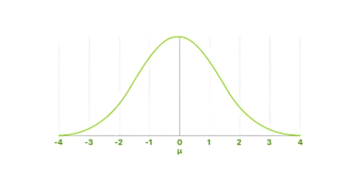
What Is the Standard Normal Distribution?
The standard normal distribution is a special type of normal distribution that has:
- Mean (μ) = 0
- Standard Deviation (σ) = 1
In simple words, it’s a normal distribution that’s been scaled and shifted so the center is at zero and the spread is exactly one unit.
Why Do We Use It?
The standard normal distribution makes it easier to:
- Compare different datasets.
- Calculate probabilities using Z-scores.
- Use statistical tables without needing a unique table for each mean and standard deviation.
Z-Score and Standard Normal
A Z-score is a way to turn any normal distribution into a standard one.
Formula: Z = (X − μ) / σ
- X = your raw score
- μ = mean of your dataset
- σ = standard deviation
The Z-score tells you how far and in what direction a value is from the mean, measured in standard deviations.
Example: Imagine student test scores have:
- Mean = 70
- Standard deviation = 10
- Your score = 85
Z = (85 − 70) / 10 = 1.5
That means you scored 1.5 standard deviations above the average. Using the standard normal table, you can find what percentage of students scored below you.
Key Takeaway
The normal distribution isn’t just a math concept; it’s a powerful tool that helps us understand patterns in everyday life. Whether you’re analyzing test scores, predicting outcomes, or making data-driven decisions, knowing how the bell curve works gives you a smarter lens to look at the world. Just remember: not all data fits the curve, so keep a critical eye and choose the right method for the right problem.